Using AIminify to compress your neural network is simple and effective. To demonstrate how it works and what your options are, we will show you how to use AIminify to compress a simple U-Net neural network.
Creating the U-Net model
To have a simple example that can easily be recreated, we chose to optimise a small U-Net model. We created U-Net models in both PyTorch and Tensorflow based on the code found here. The models were both trained for 10 epochs on the Carvana data set, which took about an hour each on a laptop with a NVIDIA GeForce RTX 4070 GPU. If you want access to the full codebase and test this yourself, please contact us.
Baseline performance
| Model type | GFLOPS | Parameters(millions) | Size | Accuracy (DICE) | Inference Time |
|---|---|---|---|---|---|
| Tensorflow | 385.530 | 31.0317 | 124.3 MB | 0.9888 | 826.2 ms |
| PyTorch | 385.629 | 31.0317 | 124.1 MB | 0.9845 | 444.4 ms |
All tests in this post have been ran on the same laptop as the models were trained on. The test set consisted of 496 images, resized to 512×512 pixels, which we processed in batches of 4. The inference time mentioned in the tables is the average inference time per image for the whole test set.
As can be seen most statistics about the baseline models are the same, except for the inference time. There can be a number of reasons for this difference, but since we’re not comparing Tensorflow to PyTorch it’s of no importance to this case study.
The baseline model accuracy is quite high, a bit over 98%, and predicts the outline of cars quite well as can be seen in the random example in Image 1.

Compressing the U-Net model
Compressing the U-Net model is now as simple as one Python command. There are however some options which have a significant impact on the output of the newly compressed model.
compressed_model, logs = minify(
    model=model,
    compression_strength=5,
    training_generator=train_set,
    validation_generator=val_set,
    loss_function=tf.keras.losses.BinaryCrossentropy(),
    quantization=False,
    fine_tune=True,
    precision="mixed",
    smart_pruning=False
)
Compression strength
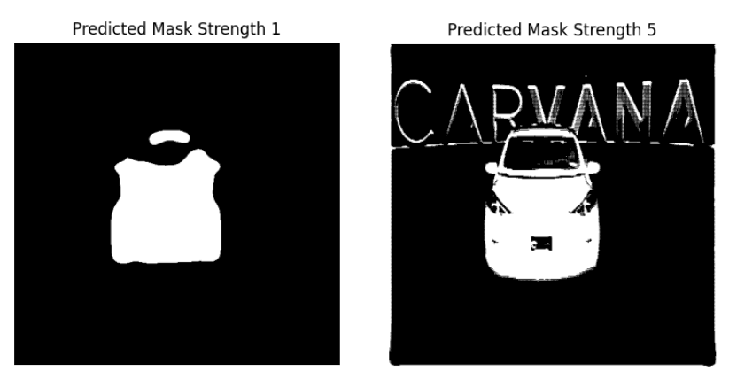
AIminify offers a compression strength of 0 to 5. This compression strength currently only influences the pruning part of the algorithm. Compression strength 0 means we do zero pruning, which can be useful if you want to do quantization only. Compression strength 1 to 5 are different settings of the pruning algorithm which respectively prune a little or a lot of the model. By adding training and validation generators and putting the fine_tune setting to true, AIminify will automatically fine-tune the model after pruning, which is needed to get it as close to the original accuracy as possible. In this example we used the option for mixed precision training as well, which basically speeds up the training time without influencing the final accuracy. In Image 2 you can see what happens if we won’t fine-tune the model and what the difference is between pruning on strength 1 and pruning on strength 5.
| Model type | Pruning Strength | Fine‑tuned | GFLOPS | Parameters (millions) | Size | Accuracy (DICE) | Inference Time |
|---|---|---|---|---|---|---|---|
| Tensorflow | 1 | Yes | 349.993 (−9.06%) | 28.2285 (−8.84%) | 113.1 MB (−9.12%) | 0.9886 (−0.02%) | 744.0 ms (−9.80%) |
| Tensorflow | 1 | No | 349.993 (−9.06%) | 28.2285 (−8.84%) | 113.1 MB (−9.12%) | 0.4084 (−58.23%) | 806.0 ms (−2.44%) |
| Tensorflow | 5 | Yes | 201.435 (−47.30%) | 16.9100 (−45.45%) | 67.8 MB (−45.62%) | 0.9890 (+0.02%) | 639.1 ms (−22.21%) |
| Tensorflow | 5 | No | 201.435 (−47.30%) | 16.9100 (−45.45%) | 67.8 MB (−45.62%) | 0.0809 (−91.93%) | 648.8 ms (−21.23%) |
| PyTorch | 1 | Yes | 347.418 (−9.79%) | 28.2098 (−9.19%) | 112.9 MB (−9.15%) | 0.9872 (+0.28%) | 464.5 ms (+4.54%) |
| PyTorch | 1 | No | 347.418 (−9.79%) | 28.2098 (−9.19%) | 112.9 MB (−9.15%) | 0.7988 (−18.53%) | 466.3 ms (+4.99%) |
| PyTorch | 5 | Yes | 196.636 (−48.90%) | 16.9012 (−45.71%) | 67.6 MB (−45.69%) | 0.9851 (+0.06%) | 290.3 ms (−34.26%) |
| PyTorch | 5 | No | 196.636 (−48.90%) | 16.9012 (−45.71%) | 67.6 MB (−45.69%) | 0.5781 (−41.82%) | 290.2 ms (−34.26%) |
From the table we can conclude multiple things:
- Pruning a model and thus reducing the amount of parameters greatly reduces the amount of GFLOPS which in turn makes inference time a lot shorter.
- Pruning can also impact the model size, cutting it almost in half.
- Pruning a model on strength 1 can already cause it to break without fine-tuning. Fine-tuning for only a few (4 in this example) epochs gets the model right back up to standard.
Quantization
Turning quantization on or off is also an important choice to make. Quantization is a big space saver and if applied well it can also improve the latency. Some models are not that suitable for quantization however and since you can’t fine-tune after quantizing it might hurt the accuracy of the model. Another tricky part of quantization is that quantized models can’t always run on the hardware that you have in mind. When the U-Net models were quantized they couldn’t run on our GPU anymore, due to various reasons that were out of scope for this project. Since comparing GPU and CPU latency is unfair, inference time is left out of this table. The number of parameters stay exactly the same, which is why they are also not shown in the table.
| Model type | Quantized | Size | Accuracy (DICE) |
|---|---|---|---|
| Tensorflow (TFLite) | Yes | 31.1 MB | 0.9865 |
| Tensorflow | No | 124.1 MB | 0.9888 |
| PyTorch | Yes | 39.6 MB | 0.9792 |
| PyTorch | No | 124.1 MB | 0.9845 |
Conclusion
In this blogpost we’ve demonstrated how easy it is to use AIminify and how we try to make the amount of options small while still keeping the user in charge of what happens with their model. We’ve shown how different parameter settings impact your model and explained what might be worth considering if you want to use these settings. Both the latency improvement and the model size reduction can be of significant help to your neural network solution. If you have any additional questions, you want to try to reproduce this example, or want to try AIminify for free on your own computer vision solution: please contact us.